> ## Documentation Index
> Fetch the complete documentation index at: https://lancedb-bcbb4faf-update-indexing-docs.mintlify.site/llms.txt
> Use this file to discover all available pages before exploring further.
# Vector Indexes
> Build and manage LanceDB vector indexes.
export const VectorIndexCustomName = "# Override the default `{column}_idx` convention by passing `name=...`.\ntable.create_index(\n metric=\"cosine\",\n vector_column_name=\"keywords_embeddings\",\n name=\"my_custom_index\",\n)\ntable.wait_for_index([\"my_custom_index\"])\nprint(table.index_stats(\"my_custom_index\"))\n";
export const VectorIndexBypassRecall = "query = np.random.random(128)\nk = 10\n\n# Ground truth: flat (exhaustive) scan, ignoring the ANN index.\ntruth = set(table.search(query).bypass_vector_index().limit(k).to_pandas()[\"id\"])\n\n# ANN results with the current nprobes setting.\nann = set(table.search(query).nprobes(20).limit(k).to_pandas()[\"id\"])\n\nrecall_at_k = len(truth & ann) / k\n";
export const VectorIndexDistanceRange = "# Only return results whose distance falls within [0.0, 0.5).\n# Useful for near-duplicate detection or thresholded similarity search.\n(\n table.search(np.random.random(128))\n .distance_range(lower_bound=0.0, upper_bound=0.5)\n .limit(10)\n .to_pandas()\n)\n";
export const VectorIndexNprobes = "# Always scan 10 partitions; scan up to 50 only if the initial pass\n# returns fewer than `limit` results (common with narrow filters).\n(\n table.search(np.random.random(128))\n .minimum_nprobes(10)\n .maximum_nprobes(50)\n .where(\"id > 100\")\n .limit(5)\n .to_pandas()\n)\n";
export const VectorIndexCheckStatus = "index_name = \"keywords_embeddings_idx\"\ntable.wait_for_index([index_name])\nprint(table.index_stats(index_name))\n";
export const VectorIndexBinarySearch = "query = np.random.randint(0, 2, size=ndim)\nquery = np.packbits(query)\ndf = table.search(query).metric(\"hamming\").limit(10).to_pandas()\ndf.vector = df.vector.apply(np.unpackbits)\n";
export const VectorIndexBinaryBuildIndex = "table.create_index(\n metric=\"hamming\",\n vector_column_name=\"vector\",\n index_type=\"IVF_FLAT\",\n)\n";
export const VectorIndexBinaryAddData = "table.add(data)\n";
export const VectorIndexBinarySchema = "table = tmp_db.create_table(table_name, schema=schema, mode=\"overwrite\")\n";
export const VectorIndexQueryHnsw = "tbl = table\ntbl.search(np.random.random((16))).limit(2).to_pandas()\n";
export const VectorIndexBuildHnsw = "table.create_index(index_type=\"IVF_HNSW_SQ\")\n";
export const VectorIndexQueryIvf = "tbl = table\ntbl.search(np.random.random((1536))).limit(2).nprobes(20).refine_factor(\n 10\n).to_pandas()\n";
export const VectorIndexAsyncConfig = "import lancedb\nimport numpy as np\nfrom lancedb.index import IvfPq\n\nasync def main():\n data = [\n {\"id\": i, \"vector\": np.random.random(8).astype(np.float32).tolist()}\n for i in range(512)\n ]\n\n db = await lancedb.connect_async(\"ex_lancedb\")\n table = await db.create_table(\n \"vector_index_async\", data=data, mode=\"overwrite\"\n )\n\n await table.create_index(\n \"vector\",\n config=IvfPq(\n distance_type=\"cosine\",\n num_partitions=16,\n num_sub_vectors=4,\n ),\n )\n return await table.list_indices()\n";
export const VectorIndexNestedField = "# The vector column `embedding` is nested inside the `image` struct.\n# Pass its full dotted path as `vector_column_name`; the same path is used\n# at query time and is what `list_indices()` reports under `columns`.\ntable.create_index(\n vector_column_name=\"image.embedding\",\n num_partitions=1,\n num_sub_vectors=1,\n name=\"image_embedding_idx\",\n)\n\nresults = (\n table.search([0.0, 1.0], vector_column_name=\"image.embedding\")\n .limit(1)\n .to_list()\n)\n";
export const VectorIndexBuildIvf = "table_name = \"vector-index-build-ivf\"\ntable = db.open_table(table_name)\ntable.create_index(\n metric=\"cosine\",\n vector_column_name=\"keywords_embeddings\",\n index_type=\"IVF_PQ\",\n)\n";
export const VectorIndexSetup = "table_name = \"vector-index-tbl\"\ntable = db.open_table(table_name)\n";
export const VectorIndexConfigureIvf = "table.create_index(metric=\"l2\", num_partitions=16, num_sub_vectors=4)\n";
Vector indexes are robust tools in facilitating fast searches across large numeric datasets.
LanceDB implements **ANN (Approximate Nearest-Neighbor)** queries with several techniques that provide benefits across a variety of use cases.
## Choosing the Right Index
LanceDB vector indexes are combined with several [quantization](/indexing/quantization) techniques to admit efficient storage.
The following table lists provided quantized vector indexes and their common use cases. You can specify index type manually in
Lance with `index_type`.
| If your priority is... | Use this index | Why | Approx. compression ratio | Python config class |
| :------------------------------------------------------- | :-------------- | :------------------------------------------ | :------------------------------------------------------------------ | :------------------ |
| Higher accuracy at small dimensions (`dimension <= 256`) | `IVF_PQ` | IVF indexing with product quantization | Usually `1/64` to `1/16` of raw size (depends on `num_sub_vectors`) | `IvfPq` |
| Maximum compression | `IVF_RQ` | IVF indexing with RaBitQ quantization | Around `1/32` of raw size | `IvfRq` |
| | `IVF_SQ` | IVF indexing with scalar quantization | Varies | `IvfSq` |
| | `IVF_HNSW_PQ` | IVF-HNSW indexing with product quantization | Varies | `IvfHnswPq` |
| Best recall/latency trade-off | `IVF_HNSW_SQ` | IVF-HNSW indexing with scalar | Typically a little larger than `1/4` of raw size | `IvfHnswSq` |
| Highest recall / no quantization | `IVF_HNSW_FLAT` | IVF-HNSW indexing with no quantization | Around raw vector size plus HNSW graph overhead | `IvfHnswFlat` |
| | `IVF_FLAT` | IVF indexing with no quantization | `1` | `IvfFlat` |
If your vector search frequently includes metadata filters (`where(...)`), use `IVF_RQ` or `IVF_PQ`. In filtered workloads, HNSW-backed IVF indexes such as `IVF_HNSW_FLAT` and `IVF_HNSW_SQ` can show higher latency variance.
## Understanding Vector Indexes
LanceDB offers two vector indexes, which can be created on any numeric Lance dataset:
**Inverted File (IVF)** and **Hierarchical Navigable Small World (HNSW)**.
### IVF
The **Inverted File Index (IVF)** accelerates ANN searches by drastically reducing the search space. The index consists of
a small set of *centroids* corresponding to an approximate solution to the
[$k$-means clustering](https://en.wikipedia.org/wiki/K-means_clustering) problem.
Each vector remembers its nearest centroid, and each centroid remembers its associated set of vectors,
called its *partition*.
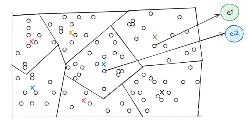 At query time, we can compare the queried vector to the smaller set of *centroids* (as opposed to the entire dataset)
for a closest match, then run a brute-force comparison against its resulting partition. This technique quickly prunes a large search space,
giving an approximate ANN result.
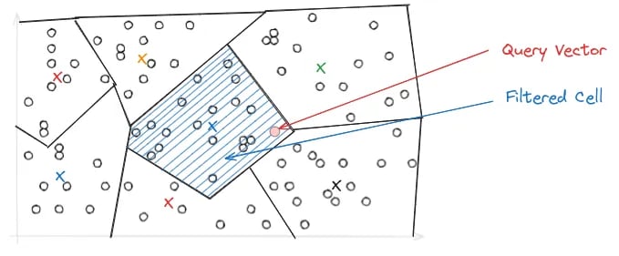
However, observe that a queried vector may lie near the boundary of $2$ or more partitions; thus, the true nearest neighbors are scattered across several different partitions.
To address this, LanceDB exposes the `nprobes` parameter, which specifies the number of partitions searched.
A high `nprobes` parameter will yield more accurate results at slightly higher runtime.
At query time, we can compare the queried vector to the smaller set of *centroids* (as opposed to the entire dataset)
for a closest match, then run a brute-force comparison against its resulting partition. This technique quickly prunes a large search space,
giving an approximate ANN result.
However, observe that a queried vector may lie near the boundary of $2$ or more partitions; thus, the true nearest neighbors are scattered across several different partitions.
To address this, LanceDB exposes the `nprobes` parameter, which specifies the number of partitions searched.
A high `nprobes` parameter will yield more accurate results at slightly higher runtime.
 ### HNSW
**Hierarchical Navigable Small World (HNSW)** constructs a layered graph hierarchy on the vector set, with edges representing distances.
We can visualize an HNSW index as a vertical stack of graphs, with the top layer having very few edges and
each other layer having a multiplicative factor more edges than the layer above it.
High layers of a HNSW hierarchy represent sparse, higher-distance networks, and lower layers represent finer, lower-distance networks.
To query a vector $q$, the index proceeds iteratively through layers, first finding $q$'s nearest neighbor in the graph, then proceeding recursively
through the induced subhierarchy until the lowest layer is reached.
### HNSW
**Hierarchical Navigable Small World (HNSW)** constructs a layered graph hierarchy on the vector set, with edges representing distances.
We can visualize an HNSW index as a vertical stack of graphs, with the top layer having very few edges and
each other layer having a multiplicative factor more edges than the layer above it.
High layers of a HNSW hierarchy represent sparse, higher-distance networks, and lower layers represent finer, lower-distance networks.
To query a vector $q$, the index proceeds iteratively through layers, first finding $q$'s nearest neighbor in the graph, then proceeding recursively
through the induced subhierarchy until the lowest layer is reached.
 To visualize this process, imagine that you must drive your car from San Francisco to a specific house in Boston. Initially, you must first drive thousands of miles
on the interstate freeway I-90 E. Eventually, you merge onto the Massachusetts Turnpike, the center
of the greater Boston highway system. From there, you use a series of increasingly smaller, narrower roads within the city (Charles River Bridge, St. Paul St,
Thatcher St) before finally reaching the house.
A key observation is that you must initially travel far distances through long-distance road networks
(the interstate freeway system), before proceeding to finer and finer road networks (greater Boston highway system, central Brookline neighborhood connectors) before finally reaching
your destination. This iterative series of road networks mimics the layered graph traversals performed by a HNSW query.
**IVF + HNSW**
In LanceDB, HNSW is not exposed as a top-level vector index. Instead, it's available as a substructure which
further indexes the selected vectors inside each IVF partition.
This combines the scalability of IVF with the high recall of HNSW.
LanceDB supports IVF-HNSW-based quantized indexes `IVF_HNSW_FLAT`, `IVF_HNSW_PQ`, and `IVF_HNSW_SQ`.
## Using Vector Indexes
Learn how to configure, build, and search LanceDB vector indexes, including build and search time parameters, asynchronous objects, and several examples.
### Configuration
#### Build-time Parameters
| Parameter | Description |
| :---------------------- | :------------------------------------------------------------------------------------------------------------------------------------------------------------------------------------------------------------------------------------------------------------------------------------------------ |
| `metric` | Default is `l2`, others available are `cosine` and `dot`. |
| `num_partitions` | The number of IVF partitions constructed (corresponds to the $k$ in $k$-means clustering). Targets roughly `sqrt(num_rows)` by default. |
| `target_partition_size` | An alternative IVF sizing knob that derives the partition count by setting the number of rows per partition. Defaults to `8192 = 2^13` for IVF-family indexes and `1,048,576 = 2^20` for IVF-HNSW-family indexes. `num_partitions` takes precedence over `target_partition_size` if both are set. |
| `num_sub_vectors` | Applies to `IVF_PQ`; defaults to `dimension // 16` (or `dimension // 8` if not a multiple of 16). Larger values produce better recall and slower search. |
| `max_iterations` | Maximum number of k-means training iterations, for every IVF/HNSW index type. Default `50`. Increase for larger datasets or to improve training quality. |
| `sample_rate` | Number of k-means training samples per partition, for every IVF/HNSW index type. Default `256`. Higher values increase both accuracy and training time. |
#### Search-time Parameters
| Parameter | Description |
| :----------------------------------------- | :--------------------------------------------------------------------------------------------------------------------------------------------------------------------------------------------------------------- |
| `limit` | Number of results to return (the `k` in `k-ANN`). |
| `nprobes` | Shorthand that sets both `minimum_nprobes` and `maximum_nprobes` to the same value. LanceDB auto-tunes this by default. |
| `minimum_nprobes` | Minimum number of partitions scanned. |
| `maximum_nprobes` | Maximum number of partitions scanned. Only scans more than `minimum_nprobes` if an initial pass does not return enough results — useful for narrow filters. Set to `0` to remove the cap. |
| `ef` | HNSW search-time exploration factor. Start around `1.5 * k` and increase up to `10 * k` for higher recall. |
| `refine_factor` | Reads and reranks additional candidates in memory to recover recall lost to quantization. |
| `distance_range(lower_bound, upper_bound)` | Return only rows whose distance falls within `[lower_bound, upper_bound)`. Either bound is optional. Useful for near-duplicate detection or "close-enough" matching. |
| `bypass_vector_index()` | Ignore the ANN index entirely and perform an exact (flat) scan. Can be used to measure ANN `recall@k`, or to query with a metric the index was not built for (e.g., a non-cosine query on a multivector column). |
**Recommended `nprobes` behavior by index type:**
| Index type | Guidance |
| :----------------------------- | :--------------------------------------------------------------------------------------------------------- |
| `IVF_HNSW_FLAT`, `IVF_HNSW_SQ` | Keep the auto-tuned `nprobes`, then tune `ef` first. Expect higher latency variance under filtered search. |
| `IVF_RQ`, `IVF_PQ` | Keep auto-tuned `nprobes`; raise only when recall is insufficient. |
**Filtered queries and adaptive `nprobes`.** When a `where(...)` filter is active, LanceDB initially scans `minimum_nprobes`
partitions and uses a wider scan if too few rows are found.
Set `minimum_nprobes == maximum_nprobes` or call `nprobes(n)` to instead fix the partition count.
Here is an example of a vector search exercising several of the above parameters.
{VectorIndexNprobes}
LanceDB also supports advanced search-time controls for thresholded retrieval, recall measurement, and working around index-level metric constraints.
**Thresholding with `distance_range`:**
{VectorIndexDistanceRange}
**Using `bypass_vector_index`:**
Use `bypass_vector_index` to compute an exact **kNN** result. Note that exact queries may be prohibitively slow on production scales.
{VectorIndexBypassRecall}
Multivector indexing currently requires `distance_type="cosine"`. Use `bypass_vector_index()` for non-`cosine` queries on a multivector column. See [Multivector Search](/search/multivector-search) for the full rules.
#### Async API and Config Objects
Create vector indexes asynchronously with `await table.create_index("vector", config=...)`. The `config` object
admits the same build-time parameters described above — pass an instance of a Python config class from the table in [Choosing the Right Index](#choosing-the-right-index):
{VectorIndexAsyncConfig}
### IVF Indexes
This example creates and queries an `IVF_PQ` index for a table of vectors with respect to `cosine` similarity.
Specify `vector_column_name` if you have multiple vector columns or non-default names.
{VectorIndexBuildIvf + VectorIndexQueryIvf}
TypeScript currently doesn't support `IvfSq` (IVF with Scalar Quantization).
For a vector field nested inside a struct, pass its full dotted path as `vector_column_name` (e.g. `image.embedding`) — the same path is used at query time and is what `list_indices()` reports under `columns`. See [Selecting the vector column](/search/vector-search#selecting-the-vector-column) for the full path syntax.
{VectorIndexNestedField}
### IVF-HNSW Indexes
Beyond the general build-time parameters above, two additional parameters are specific to IVF-HNSW indexes:
| Parameter | Description |
| :---------------- | :-------------------------------------------------------------------------------------------------------------------------------------------------------- |
| `m` | The number of neighbors to select for each vector in the HNSW graph. |
| `ef_construction` | The number of candidates to evaluate during the construction of the HNSW graph. Start at `150`; increase for better recall, decrease for faster indexing. |
Partition sizing follows the general `num_partitions`/`target_partition_size` guidance above.
The snippet below builds and queries an `IVF_HNSW_SQ` index.
{VectorIndexBuildHnsw + VectorIndexQueryHnsw}
### Managing Vector Indexes
Enterprise-only
In LanceDB Enterprise, vector indexes are managed **automatically**. The system asynchronously updates and optimizes indexes as a background process:
* Automatically manages indexing parameters and storage
* Infers vector columns from the schema
Open-Source
LanceDB OSS users can manually create vector indexes by calling `table.create_index()`.
See the above sections for guidance on manually tuning index parameters as data changes.
`create_index()` returns immediately, but the vector index builds asynchronously.
To wait until all data is indexed, specify the `wait_timeout` parameter, or call `wait_for_index(...)` afterward —
it waits for the named index to exist and for `index_stats(...)` to report `num_unindexed_rows == 0`.
Rows appended after an initial index build remain outside the index until refreshed manually (OSS) or automatically (Enterprise). Normal
search still checks those unindexed rows with a slower fallback path; `fast_search()` skips that
fallback and searches only indexed rows.
**Operational checks**
After appends or other writes, use `optimize()` to fold new rows into existing indexes.
#### Check Index Status
Vector index creation runs in the background and may take some time to complete.
While it is ongoing, you can check its status through the API or the **LanceDB Enterprise UI**.
In the LanceDB Enterprise UI, navigate to your table page - the "Index" column reflects each column's index status: it is blank when no index exists, shows an "in progress" label while the index is being built, and shows the index type once the build completes.
To check status programmatically, use `list_indices()` and `index_stats()`. **By default**, the index name is formed by appending `_idx` to the column name (e.g., a `keywords_embeddings` column produces `keywords_embeddings_idx`). Note that `list_indices()` only returns information after the index is fully built.
Each entry returned by `list_indices()` also carries detailed per-index metadata, so you can inspect an index without a follow-up `index_stats()` call. Node.js exposes the same fields in camelCase (`num_indexed_rows` → `numIndexedRows`):
| Parameter | Description |
| :--------------------------------------- | :------------------------------------------------------------------------- |
| `num_indexed_rows`, `num_unindexed_rows` | Index coverage over the table |
| `size_bytes` | Total size of the index files on disk |
| `num_segments`, `index_version` | On-disk layout and format version |
| `created_at` | Creation time (ms since the Unix epoch in Node.js) |
| `index_uuid`, `type_url` | Internal identifiers for the index segment |
| `index_details` | Type-specific details (e.g. IVF partition counts or quantization settings) |
{VectorIndexCheckStatus}
These fields are populated for local and embedded tables. On LanceDB Enterprise remote tables they are returned as `None` / `undefined` until the server response surfaces them.
#### Custom Index Names
The `{column}_idx` suffix is the default naming convetion.
Pass `name=...` to `create_index()` to override it. Once set, the custom name will be reflected in `list_indices()`, `index_stats(name)`, and `wait_for_index([name])`.
{VectorIndexCustomName}
To visualize this process, imagine that you must drive your car from San Francisco to a specific house in Boston. Initially, you must first drive thousands of miles
on the interstate freeway I-90 E. Eventually, you merge onto the Massachusetts Turnpike, the center
of the greater Boston highway system. From there, you use a series of increasingly smaller, narrower roads within the city (Charles River Bridge, St. Paul St,
Thatcher St) before finally reaching the house.
A key observation is that you must initially travel far distances through long-distance road networks
(the interstate freeway system), before proceeding to finer and finer road networks (greater Boston highway system, central Brookline neighborhood connectors) before finally reaching
your destination. This iterative series of road networks mimics the layered graph traversals performed by a HNSW query.
**IVF + HNSW**
In LanceDB, HNSW is not exposed as a top-level vector index. Instead, it's available as a substructure which
further indexes the selected vectors inside each IVF partition.
This combines the scalability of IVF with the high recall of HNSW.
LanceDB supports IVF-HNSW-based quantized indexes `IVF_HNSW_FLAT`, `IVF_HNSW_PQ`, and `IVF_HNSW_SQ`.
## Using Vector Indexes
Learn how to configure, build, and search LanceDB vector indexes, including build and search time parameters, asynchronous objects, and several examples.
### Configuration
#### Build-time Parameters
| Parameter | Description |
| :---------------------- | :------------------------------------------------------------------------------------------------------------------------------------------------------------------------------------------------------------------------------------------------------------------------------------------------ |
| `metric` | Default is `l2`, others available are `cosine` and `dot`. |
| `num_partitions` | The number of IVF partitions constructed (corresponds to the $k$ in $k$-means clustering). Targets roughly `sqrt(num_rows)` by default. |
| `target_partition_size` | An alternative IVF sizing knob that derives the partition count by setting the number of rows per partition. Defaults to `8192 = 2^13` for IVF-family indexes and `1,048,576 = 2^20` for IVF-HNSW-family indexes. `num_partitions` takes precedence over `target_partition_size` if both are set. |
| `num_sub_vectors` | Applies to `IVF_PQ`; defaults to `dimension // 16` (or `dimension // 8` if not a multiple of 16). Larger values produce better recall and slower search. |
| `max_iterations` | Maximum number of k-means training iterations, for every IVF/HNSW index type. Default `50`. Increase for larger datasets or to improve training quality. |
| `sample_rate` | Number of k-means training samples per partition, for every IVF/HNSW index type. Default `256`. Higher values increase both accuracy and training time. |
#### Search-time Parameters
| Parameter | Description |
| :----------------------------------------- | :--------------------------------------------------------------------------------------------------------------------------------------------------------------------------------------------------------------- |
| `limit` | Number of results to return (the `k` in `k-ANN`). |
| `nprobes` | Shorthand that sets both `minimum_nprobes` and `maximum_nprobes` to the same value. LanceDB auto-tunes this by default. |
| `minimum_nprobes` | Minimum number of partitions scanned. |
| `maximum_nprobes` | Maximum number of partitions scanned. Only scans more than `minimum_nprobes` if an initial pass does not return enough results — useful for narrow filters. Set to `0` to remove the cap. |
| `ef` | HNSW search-time exploration factor. Start around `1.5 * k` and increase up to `10 * k` for higher recall. |
| `refine_factor` | Reads and reranks additional candidates in memory to recover recall lost to quantization. |
| `distance_range(lower_bound, upper_bound)` | Return only rows whose distance falls within `[lower_bound, upper_bound)`. Either bound is optional. Useful for near-duplicate detection or "close-enough" matching. |
| `bypass_vector_index()` | Ignore the ANN index entirely and perform an exact (flat) scan. Can be used to measure ANN `recall@k`, or to query with a metric the index was not built for (e.g., a non-cosine query on a multivector column). |
**Recommended `nprobes` behavior by index type:**
| Index type | Guidance |
| :----------------------------- | :--------------------------------------------------------------------------------------------------------- |
| `IVF_HNSW_FLAT`, `IVF_HNSW_SQ` | Keep the auto-tuned `nprobes`, then tune `ef` first. Expect higher latency variance under filtered search. |
| `IVF_RQ`, `IVF_PQ` | Keep auto-tuned `nprobes`; raise only when recall is insufficient. |
**Filtered queries and adaptive `nprobes`.** When a `where(...)` filter is active, LanceDB initially scans `minimum_nprobes`
partitions and uses a wider scan if too few rows are found.
Set `minimum_nprobes == maximum_nprobes` or call `nprobes(n)` to instead fix the partition count.
Here is an example of a vector search exercising several of the above parameters.
{VectorIndexNprobes}
LanceDB also supports advanced search-time controls for thresholded retrieval, recall measurement, and working around index-level metric constraints.
**Thresholding with `distance_range`:**
{VectorIndexDistanceRange}
**Using `bypass_vector_index`:**
Use `bypass_vector_index` to compute an exact **kNN** result. Note that exact queries may be prohibitively slow on production scales.
{VectorIndexBypassRecall}
Multivector indexing currently requires `distance_type="cosine"`. Use `bypass_vector_index()` for non-`cosine` queries on a multivector column. See [Multivector Search](/search/multivector-search) for the full rules.
#### Async API and Config Objects
Create vector indexes asynchronously with `await table.create_index("vector", config=...)`. The `config` object
admits the same build-time parameters described above — pass an instance of a Python config class from the table in [Choosing the Right Index](#choosing-the-right-index):
{VectorIndexAsyncConfig}
### IVF Indexes
This example creates and queries an `IVF_PQ` index for a table of vectors with respect to `cosine` similarity.
Specify `vector_column_name` if you have multiple vector columns or non-default names.
{VectorIndexBuildIvf + VectorIndexQueryIvf}
TypeScript currently doesn't support `IvfSq` (IVF with Scalar Quantization).
For a vector field nested inside a struct, pass its full dotted path as `vector_column_name` (e.g. `image.embedding`) — the same path is used at query time and is what `list_indices()` reports under `columns`. See [Selecting the vector column](/search/vector-search#selecting-the-vector-column) for the full path syntax.
{VectorIndexNestedField}
### IVF-HNSW Indexes
Beyond the general build-time parameters above, two additional parameters are specific to IVF-HNSW indexes:
| Parameter | Description |
| :---------------- | :-------------------------------------------------------------------------------------------------------------------------------------------------------- |
| `m` | The number of neighbors to select for each vector in the HNSW graph. |
| `ef_construction` | The number of candidates to evaluate during the construction of the HNSW graph. Start at `150`; increase for better recall, decrease for faster indexing. |
Partition sizing follows the general `num_partitions`/`target_partition_size` guidance above.
The snippet below builds and queries an `IVF_HNSW_SQ` index.
{VectorIndexBuildHnsw + VectorIndexQueryHnsw}
### Managing Vector Indexes
Enterprise-only
In LanceDB Enterprise, vector indexes are managed **automatically**. The system asynchronously updates and optimizes indexes as a background process:
* Automatically manages indexing parameters and storage
* Infers vector columns from the schema
Open-Source
LanceDB OSS users can manually create vector indexes by calling `table.create_index()`.
See the above sections for guidance on manually tuning index parameters as data changes.
`create_index()` returns immediately, but the vector index builds asynchronously.
To wait until all data is indexed, specify the `wait_timeout` parameter, or call `wait_for_index(...)` afterward —
it waits for the named index to exist and for `index_stats(...)` to report `num_unindexed_rows == 0`.
Rows appended after an initial index build remain outside the index until refreshed manually (OSS) or automatically (Enterprise). Normal
search still checks those unindexed rows with a slower fallback path; `fast_search()` skips that
fallback and searches only indexed rows.
**Operational checks**
After appends or other writes, use `optimize()` to fold new rows into existing indexes.
#### Check Index Status
Vector index creation runs in the background and may take some time to complete.
While it is ongoing, you can check its status through the API or the **LanceDB Enterprise UI**.
In the LanceDB Enterprise UI, navigate to your table page - the "Index" column reflects each column's index status: it is blank when no index exists, shows an "in progress" label while the index is being built, and shows the index type once the build completes.
To check status programmatically, use `list_indices()` and `index_stats()`. **By default**, the index name is formed by appending `_idx` to the column name (e.g., a `keywords_embeddings` column produces `keywords_embeddings_idx`). Note that `list_indices()` only returns information after the index is fully built.
Each entry returned by `list_indices()` also carries detailed per-index metadata, so you can inspect an index without a follow-up `index_stats()` call. Node.js exposes the same fields in camelCase (`num_indexed_rows` → `numIndexedRows`):
| Parameter | Description |
| :--------------------------------------- | :------------------------------------------------------------------------- |
| `num_indexed_rows`, `num_unindexed_rows` | Index coverage over the table |
| `size_bytes` | Total size of the index files on disk |
| `num_segments`, `index_version` | On-disk layout and format version |
| `created_at` | Creation time (ms since the Unix epoch in Node.js) |
| `index_uuid`, `type_url` | Internal identifiers for the index segment |
| `index_details` | Type-specific details (e.g. IVF partition counts or quantization settings) |
{VectorIndexCheckStatus}
These fields are populated for local and embedded tables. On LanceDB Enterprise remote tables they are returned as `None` / `undefined` until the server response surfaces them.
#### Custom Index Names
The `{column}_idx` suffix is the default naming convetion.
Pass `name=...` to `create_index()` to override it. Once set, the custom name will be reflected in `list_indices()`, `index_stats(name)`, and `wait_for_index([name])`.
{VectorIndexCustomName}